ルジャンドル多項式 (ルジャンドルたこうしき、英 : Legendre polynomial )とは、ルジャンドルの微分方程式 を満たすルジャンドル関数 のうち次数が非負整数 のものを言う。直交多項式 の一種である。
定義 解析学 においてルジャンドルの微分方程式
d d x [ ( 1 − x 2 ) d d x f ( x ) ] + λ ( λ + 1 ) f ( x ) = 0 {\displaystyle {\mathrm {d} \over \mathrm {d} x}\left[(1-x^{2}){\mathrm {d} \over \mathrm {d} x}f(x)\right]+\lambda (\lambda +1)f(x)=0} (λ は任意の複素数 とする)は標準的な冪級数 法を用いて解けることが知られており、その解は一般にルジャンドル関数 と呼ばれる(何れもアドリアン=マリ・ルジャンドル に名を因む)。この方程式は x = ±1確定特異点(英語版) を持つから、一般には原点の周りでの級数解の収束半径 は 1 である。
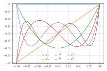
n = 5 までのルジャンドル多項式のグラフλ が非負整数 n = 0, 1, 2, …x = ±1x = 1初期条件 を課すと、解は一意に定まる。これを n 次のルジャンドル多項式 と呼び、普通は P n x )[1] n 次のルジャンドル多項式全体が成す関数族を総称的にルジャンドル多項式 と呼ぶ。ルジャンドル多項式は後述する関数空間 の内積 に関して直交系 を成す。ただし、この内積についての各 P n x )P n 正規直交系 にはなっていない点は注意を要する。各ルジャンドル多項式 P n x )n 次多項式で、ロドリゲスの公式
P n ( x ) = 1 2 n n ! d n d x n [ ( x 2 − 1 ) n ] {\displaystyle P_{n}(x)={1 \over 2^{n}n!}{\mathrm {d} ^{n} \over \mathrm {d} x^{n}}\left[(x^{2}-1)^{n}\right]} で表すことができる。
ルジャンドル多項式がルジャンドルの微分方程式を満たすことは、恒等式
( x 2 − 1 ) d d x ( x 2 − 1 ) n = 2 n x ( x 2 − 1 ) n {\displaystyle (x^{2}-1){\frac {\mathrm {d} }{\mathrm {d} x}}(x^{2}-1)^{n}=2nx(x^{2}-1)^{n}} の両辺を n + 1 一般ライプニッツ則 を適用すればわかる[2] P n テイラー級数
1 1 − 2 x t + t 2 = ∑ n = 0 ∞ P n ( x ) t n {\displaystyle {\frac {1}{\sqrt {1-2xt+t^{2}}}}=\sum _{n=0}^{\infty }P_{n}(x)t^{n}}
(1 )
の係数として定義することもできる[3] 母函数 は物理学 において多重極展開(英語版) に利用される。
帰納的定義 上記の式 (1)
P 0 ( x ) = 1 , P 1 ( x ) = x {\displaystyle P_{0}(x)=1,P_{1}(x)=x} となることがわかる。残りの多項式を得るのには、上記のテイラー展開を直截に計算するよりも、ボネの漸化式
( n + 1 ) P n + 1 ( x ) = ( 2 n + 1 ) x P n ( x ) − n P n − 1 ( x ) {\displaystyle (n+1)P_{n+1}(x)=(2n+1)xP_{n}(x)-nP_{n-1}(x)} を用いるのが適当である。この漸化式 は、式 (1) t に関して微分したものを整理して得られる等式
x − t 1 − 2 x t + t 2 = ( 1 − 2 x t + t 2 ) ∑ n = 1 ∞ n P n ( x ) t n − 1 {\displaystyle {\frac {x-t}{\sqrt {1-2xt+t^{2}}}}=(1-2xt+t^{2})\sum _{n=1}^{\infty }nP_{n}(x)t^{n-1}} の分母に現れる平方根を式 (1) t の冪に対する係数比較(英語版) を行えば得られる。漸化式に初期条件としてすでに得られている P 0 , P 1
漸化式を解いて陽に表せば
P n ( x ) = 1 2 n ∑ k = 0 n ( n k ) 2 ( x − 1 ) n − k ( x + 1 ) k = ∑ k = 0 n ( n k ) ( − n − 1 k ) ( 1 − x 2 ) k = 2 n ⋅ ∑ k = 0 n x k ( n k ) ( n + k − 1 2 n ) {\displaystyle {\begin{aligned}P_{n}(x)&={\frac {1}{2^{n}}}\sum _{k=0}^{n}{n \choose k}^{2}(x-1)^{n-k}(x+1)^{k}\\&=\sum _{k=0}^{n}{n \choose k}{-n-1 \choose k}\left({\frac {1-x}{2}}\right)^{k}\\&=2^{n}\cdot \sum _{k=0}^{n}x^{k}{n \choose k}{{\frac {n+k-1}{2}} \choose n}\end{aligned}}} などのように書くことができる。後段はルジャンドル多項式を単に単項式として表して二項係数 の乗法公式を使えば、漸化式から直ちに得られる。
具体的に最初のいくつかのルジャンドル多項式を挙げれば以下のようになる:
n P n ( x ) {\displaystyle P_{n}(x)} 0 1 {\displaystyle 1} 1 x {\displaystyle x} 2 1 2 ( 3 x 2 − 1 ) {\displaystyle \textstyle {\frac {1}{2}}(3x^{2}-1)} 3 1 2 ( 5 x 3 − 3 x ) {\displaystyle \textstyle {\frac {1}{2}}(5x^{3}-3x)} 4 1 8 ( 35 x 4 − 30 x 2 + 3 ) {\displaystyle \textstyle {\frac {1}{8}}(35x^{4}-30x^{2}+3)} 5 1 8 ( 63 x 5 − 70 x 3 + 15 x ) {\displaystyle \textstyle {\frac {1}{8}}(63x^{5}-70x^{3}+15x)} 6 1 16 ( 231 x 6 − 315 x 4 + 105 x 2 − 5 ) {\displaystyle \textstyle {\frac {1}{16}}(231x^{6}-315x^{4}+105x^{2}-5)} 7 1 16 ( 429 x 7 − 693 x 5 + 315 x 3 − 35 x ) {\displaystyle \textstyle {\frac {1}{16}}(429x^{7}-693x^{5}+315x^{3}-35x)} 8 1 128 ( 6435 x 8 − 12012 x 6 + 6930 x 4 − 1260 x 2 + 35 ) {\displaystyle \textstyle {\frac {1}{128}}(6435x^{8}-12012x^{6}+6930x^{4}-1260x^{2}+35)} 9 1 128 ( 12155 x 9 − 25740 x 7 + 18018 x 5 − 4620 x 3 + 315 x ) {\displaystyle \textstyle {\frac {1}{128}}(12155x^{9}-25740x^{7}+18018x^{5}-4620x^{3}+315x)} 10 1 256 ( 46189 x 10 − 109395 x 8 + 90090 x 6 − 30030 x 4 + 3465 x 2 − 63 ) {\displaystyle \textstyle {\frac {1}{256}}(46189x^{10}-109395x^{8}+90090x^{6}-30030x^{4}+3465x^{2}-63)}
直交性 ルジャンドル多項式の重要な性質の一つは、これらが閉区間 [−1, 1] 上の L 2 -内積に関して直交 すること、即ち以下の式を満たすことである。
∫ − 1 1 P m ( x ) P n ( x ) d x = 2 2 n + 1 δ m n {\displaystyle \int _{-1}^{1}P_{m}(x)P_{n}(x)~\mathrm {d} x={2 \over {2n+1}}\delta _{mn}} ここで δ mn クロネッカーのデルタ 、即ち m = n x , x 2 ,...} にシュミットの直交化法 を適用することによってルジャンドル多項式を導出法とすることが可能である。この直交性により、ルジャンドル多項式系がエルミート 微分作用素
d d x [ ( 1 − x 2 ) d d x P ( x ) ] = − λ P ( x ) {\displaystyle {\mathrm {d} \over \mathrm {d} x}\left[(1-x^{2}){\mathrm {d} \over \mathrm {d} x}P(x)\right]=-\lambda P(x)} の固有値 λ = n (n + 1)固有関数 系となるようなスツルム・リウヴィル理論 としてルジャンドルの微分方程式を捉えることができる。
物理学における応用 ルジャンドル多項式は初め、1782年にアドリアン=マリ・ルジャンドル [4] ニュートン・ポテンシャル(英語版)
1 | x − x ′ | = 1 r 2 + r ′ 2 − 2 r r ′ cos γ = ∑ ℓ = 0 ∞ r ′ ℓ r ℓ + 1 P ℓ ( cos γ ) {\displaystyle {\frac {1}{\left|{\boldsymbol {x}}-{\boldsymbol {x}}^{\prime }\right|}}={\frac {1}{\sqrt {r^{2}+r^{\prime 2}-2rr'\cos \gamma }}}=\sum _{\ell =0}^{\infty }{\frac {r^{\prime \ell }}{r^{\ell +1}}}P_{\ell }(\cos \gamma )} の展開の係数として定義された。ここに、r , r ′x x γ はそれらのベクトルのなす角である。上記の級数は r > r ′質点 に対応する重力ポテンシャル もしくは点電荷 に対応するクーロンポテンシャル を極座標表示する際に用いることができる。このルジャンドル多項式を用いた展開は、例えば連続質量や電荷分布の上でこの展開を積分するときなどに有用である。
ルジャンドル多項式は、空間の無電荷領域における電位 に関するラプラス方程式
∇ 2 Φ ( x ) = 0 {\displaystyle \nabla ^{2}\Phi ({\boldsymbol {x}})=0} を軸対称な(方位角 に依存しない)境界条件 のもとで、変数分離法 を用いて解く際にも登場する。ここで、 ˆ z θ を観測者の位置と ˆ z
Φ ( r , θ ) = ∑ ℓ = 0 ∞ [ A ℓ r ℓ + B ℓ r − ( ℓ + 1 ) ] P ℓ ( cos θ ) {\displaystyle \Phi (r,\theta )=\sum _{\ell =0}^{\infty }\left[A_{\ell }r^{\ell }+B_{\ell }r^{-(\ell +1)}\right]P_{\ell }(\cos \theta )} となる。A ℓ B ℓ [5]
三次元における中心力 に対するシュレーディンガー方程式を解く際にもルジャンドル多項式は現れる。
多重極展開におけるルジャンドル多項式 Figure 2 ルジャンドル多項式は、多重極展開で自然に現れる
1 1 + η 2 − 2 η x = ∑ k = 0 ∞ η k P k ( x ) {\displaystyle {\frac {1}{\sqrt {1+\eta ^{2}-2\eta x}}}=\sum _{k=0}^{\infty }\eta ^{k}P_{k}(x)} なる形の関数(記号を少し変えてあるが、上で述べたものと同じ)の展開においても有用である。等式の左辺はルジャンドル多項式の母関数 の閉じた形である。
例として、(球座標系 での)電位 Φ(r , θ ) が z -軸上の点 z = a 点電荷 によるものとすれば、
Φ ( r , θ ) ∝ 1 R = 1 r 2 + a 2 − 2 a r cos θ {\displaystyle \Phi (r,\theta )\propto {\frac {1}{R}}={\frac {1}{\sqrt {r^{2}+a^{2}-2ar\cos \theta }}}} と書くことができる。観測点 P の半径 r が a より大きければ、電位はルジャンドル多項式を用いて
Φ ( r , θ ) ∝ 1 r ∑ k = 0 ∞ ( a r ) k P k ( cos θ ) {\displaystyle \Phi (r,\theta )\propto {\frac {1}{r}}\sum _{k=0}^{\infty }\left({\frac {a}{r}}\right)^{k}P_{k}(\cos \theta )} と展開することができる。ここでは η = a /r < 1x = cosθ
逆に、観測点 P の半径 r が a より小さいならば、電位を上記のようにルジャンドル多項式展開することはできるが、a と r とは入れ替わる。この展開は内部多重極展開 (interior multipole expansion ) の基本となる。
その他の性質 ルジャンドル多項式は対称または反対称、即ち
P n ( − x ) = ( − 1 ) n P n ( x ) {\displaystyle P_{n}(-x)=(-1)^{n}P_{n}(x)} を満たす[6]
微分方程式と直交性はスケール変換に依らない性質だから、ルジャンドル多項式はその定義において適当に定数倍して
P k ( 1 ) = 1 {\displaystyle P_{k}(1)=1} を満たすように「標準化」される(「正規化」とも言うが、実際にノルムが 1 というわけではないので紛らわしい)。端点における微分係数は
P k ′ ( 1 ) = k ( k + 1 ) 2 {\displaystyle P_{k}'(1)={\frac {k(k+1)}{2}}} で与えられる。既に述べたとおり、ルジャンドル多項式はボネの漸化式と呼ばれる三項間漸化式
( n + 1 ) P n + 1 ( x ) = ( 2 n + 1 ) x P n ( x ) − n P n − 1 ( x ) {\displaystyle (n+1)P_{n+1}(x)=(2n+1)xP_{n}(x)-nP_{n-1}(x)} と、公式
x 2 − 1 n d d x P n ( x ) = x P n ( x ) − P n − 1 ( x ) {\displaystyle {\frac {x^{2}-1}{n}}{\frac {\mathrm {d} }{\mathrm {d} x}}P_{n}(x)=xP_{n}(x)-P_{n-1}(x)} に従うが、これらから得られる等式
( 2 n + 1 ) P n ( x ) = d d x [ P n + 1 ( x ) − P n − 1 ( x ) ] {\displaystyle (2n+1)P_{n}(x)={\frac {\mathrm {d} }{\mathrm {d} x}}\left[P_{n+1}(x)-P_{n-1}(x)\right]} ルジャンドル多項式の積分に有効である。これを繰り返し用いて
d d x P n + 1 ( x ) = ( 2 n + 1 ) P n ( x ) + ( 2 ( n − 2 ) + 1 ) P n − 2 ( x ) + ( 2 ( n − 4 ) + 1 ) P n − 4 ( x ) + ⋯ {\displaystyle {\frac {\mathrm {d} }{\mathrm {d} x}}P_{n+1}(x)=(2n+1)P_{n}(x)+(2(n-2)+1)P_{n-2}(x)+(2(n-4)+1)P_{n-4}(x)+\dotsb } あるいは同じことだが、
d d x P n + 1 ( x ) = 2 P n ( x ) ‖ P n ( x ) ‖ 2 + 2 P n − 2 ( x ) ‖ P n − 2 ( x ) ‖ 2 + ⋯ {\displaystyle {\mathrm {d} \over \mathrm {d} x}P_{n+1}(x)={2P_{n}(x) \over \|P_{n}(x)\|^{2}}+{2P_{n-2}(x) \over \|P_{n-2}(x)\|^{2}}+\dotsb } が得られる。ただし、ǁP n x )ǁ は閉区間 [−1, 1] 上のノルム
‖ P n ( x ) ‖ = ∫ − 1 1 ( P n ( x ) ) 2 d x = 2 2 n + 1 {\displaystyle \|P_{n}(x)\|={\sqrt {\int _{-1}^{1}(P_{n}(x))^{2}\,\mathrm {d} x}}={\sqrt {\frac {2}{2n+1}}}} である。ボネの漸化式から帰納的に陽な表現
P n ( x ) = ∑ k = 0 n ( − 1 ) k ( n k ) 2 ( 1 + x 2 ) n − k ( 1 − x 2 ) k {\displaystyle P_{n}(x)=\sum _{k=0}^{n}(-1)^{k}{\binom {n}{k}}^{2}\left({\frac {1+x}{2}}\right)^{n-k}\left({\frac {1-x}{2}}\right)^{k}} が得られる。ルジャンドル多項式に対するアスキー-ギャスパーの不等式(英語版) は
∑ j = 0 n P j ( x ) ≥ 0 ( x ≥ − 1 ) {\displaystyle \sum _{j=0}^{n}P_{j}(x)\geq 0\qquad (x\geq -1)} を導く。
ずらしルジャンドル多項式 ずらしルジャンドル多項式 (shifted Legendre polynomial ) は
P ~ n ( x ) = P n ( 2 x − 1 ) {\displaystyle {\tilde {P}}_{n}(x)=P_{n}(2x-1)} で定義される。ここで、ずらし写像(実はアフィン変換 )x ↦ 2x − 1[0, 1] を区間 [−1, 1] へ写す全単射 として選ばれたもので、それゆえ多項式系 ~ P n x )[0, 1] 上での直交性
∫ 0 1 P m ~ ( x ) P n ~ ( x ) d x = 1 2 n + 1 δ m n {\displaystyle \int _{0}^{1}{\tilde {P_{m}}}(x){\tilde {P_{n}}}(x)\,\mathrm {d} x={1 \over {2n+1}}\delta _{mn}} が従う。ずらしルジャンドル多項式の明示式は
P n ~ ( x ) = ( − 1 ) n ∑ k = 0 n ( n k ) ( n + k k ) ( − x ) k {\displaystyle {\tilde {P_{n}}}(x)=(-1)^{n}\sum _{k=0}^{n}{n \choose k}{n+k \choose k}(-x)^{k}} で与えられる。ロドリゲスの公式 のずらしルジャンドル多項式版は
P n ~ ( x ) = 1 n ! d n d x n [ ( x 2 − x ) n ] {\displaystyle {\tilde {P_{n}}}(x)={\frac {1}{n!}}{\mathrm {d} ^{n} \over \mathrm {d} x^{n}}\left[(x^{2}-x)^{n}\right]} となる。ずらしルジャンドル多項式の最初の方のいくつかは以下のようになる。
n P n ~ ( x ) {\displaystyle {\tilde {P_{n}}}(x)} 0 1 1 2 x − 1 {\displaystyle 2x-1} 2 6 x 2 − 6 x + 1 {\displaystyle 6x^{2}-6x+1} 3 20 x 3 − 30 x 2 + 12 x − 1 {\displaystyle 20x^{3}-30x^{2}+12x-1}
詳細は「en:Associated Legendre polynomials」を参照
非負整数 k 、m で
k ≧ m を満たすものに対し、ルジャンドル陪多項式 P k m t )
P k m ( t ) = 1 2 k ( 1 − t 2 ) m / 2 ∑ j = 0 ⌊ ( k − m ) / 2 ⌋ ( − 1 ) j ( 2 k − 2 j ) ! j ! ( k − j ) ! ( k − 2 j − m ) ! t k − 2 j − m {\displaystyle P_{k}{}^{m}(t)={\frac {1}{2^{k}}}(1-t^{2})^{m/2}\sum _{j=0}^{\lfloor (k-m)/2\rfloor }{(-1)^{j}(2k-2j)! \over j!(k-j)!(k-2j-m)!}t^{k-2j-m}} と定義する[7] P k m t )ルジャンドルの陪微分方程式
( 1 − t 2 ) y ″ ( t ) − 2 t y ′ ( t ) + ( k ( k + 1 ) − m 2 1 − t 2 ) y ( t ) = 0 {\displaystyle (1-t^{2})y''(t)-2ty'(t)+\left(k(k+1)-{m^{2} \over 1-t^{2}}\right)y(t)=0} の解である。なお、ルジャンドルの陪微分方程式は k ≧ m Yk m (θ , φ )
P k m t )P k t )
P k m ( t ) = ( 1 − t 2 ) m / 2 d m P k ( t ) d t m {\displaystyle P_{k}{}^{m}(t)=(1-t^{2})^{m/2}{\frac {\mathrm {d} ^{m}P_{k}(t)}{\mathrm {d} t^{m}}}} 関連項目 脚注 [脚注の使い方 ]
出典 ^ 永宮健夫 『応用微分方程式論』、共立出版社、1967年、pp46-52。 ^ Courant & Hilbert 1953 , II, §8^ George B. Arfken, Hans J. Weber (2005), Mathematical Methods for Physicists , Elsevier Academic Press, p. 743, ISBN 0-12-059876-0, https://books.google.fr/books?id=qLFo_Z-PoGIC&printsec=frontcover&hl=ja&source=gbs_ge_summary_r&cad=0#v=onepage&q&f=false ^ M. Le Gendre, “Recherches sur l'attraction des sphéroïdes homogènes”, Mémoires de Mathématiques et de Physique, présentés à l'Académie Royale des Sciences, par divers savans, et lus dans ses Assemblées , Tome X, pp. 411-435 (Paris, 1785). [注: ルジャンドルは彼の発見を1782年に科学アカデミーに提出したが、出版されたのは1785年であった。] ^ Jackson, J.D. Classical Electrodynamics , 3rd edition, Wiley & Sons, 1999. page 103 ^ George B. Arfken, Hans J. Weber (2005), Mathematical Methods for Physicists , Elsevier Academic Press, p. 753, ISBN 0-12-059876-0, https://books.google.fr/books?id=qLFo_Z-PoGIC&printsec=frontcover&hl=ja&source=gbs_ge_summary_r&cad=0#v=onepage&q&f=false ^ 日本測地学会 2004 参考文献 Abramowitz, Milton; Stegun, Irene A. (1965), Handbook of Mathematical Functions with Formulas, Graphs, and Mathematical Tables ISBN 978-0486612720 Bayin, S.S. (2006), Mathematical Methods in Science and Engineering , Wiley Belousov, S. L. (1962), Tables of normalized associated Legendre polynomials , Mathematical tables, 18 , Pergamon Press Courant, Richard ; Hilbert, David (1953), Methods of Mathematical Physics, Volume 1 , New York: Interscience Publischer, Inc Dunster, T. M. (2010), “Legendre and Related Functions”, in Olver, Frank W. J.; Lozier, Daniel M.; Boisvert, Ronald F. et al., NIST Handbook of Mathematical Functions ISBN 978-0521192255, http://dlmf.nist.gov/14 Koornwinder, Tom H.; Wong, Roderick S. C.; Koekoek, Roelof; Swarttouw, René F. (2010), “Orthogonal Polynomials”, in Olver, Frank W. J.; Lozier, Daniel M.; Boisvert, Ronald F. et al., NIST Handbook of Mathematical Functions ISBN 978-0521192255, http://dlmf.nist.gov/18 Refaat El Attar (2009), Legendre Polynomials and Functions , CreateSpace, ISBN 978-1-4414-9012-4 高知大学自然科学系 田部井隆雄、神奈川県温泉地学研究所 里村幹夫、京都大学大学院理学研究科 福田洋一 (2004年). “4-4. ルジャンドルの多項式, 陪多項式”. 日本測地学会. 2017年1月4日 閲覧。 外部リンク A quick informal derivation of the Legendre polynomial in the context of the quantum mechanics of hydrogen Hazewinkel, Michiel, ed. (2001), “Legendre polynomials”, Encyclopedia of Mathematics , Springer, ISBN 978-1-55608-010-4, https://www.encyclopediaofmath.org/index.php?title=Legendre_polynomials Wolfram MathWorld entry on Legendre polynomials Module for Legendre Polynomials by John H. Mathews Dr James B. Calvert's article on Legendre polynomials from his personal collection of mathematics The Legendre Polynomials by Carlyle E. Moore Legendre Polynomials from Hyperphysics 典拠管理データベース
全般 国立図書館 フランス BnF data ドイツ イスラエル アメリカ 日本 チェコ その他
![{\displaystyle {\mathrm {d} \over \mathrm {d} x}\left[(1-x^{2}){\mathrm {d} \over \mathrm {d} x}f(x)\right]+\lambda (\lambda +1)f(x)=0}](https://wikimedia.org/api/rest_v1/media/math/render/svg/05e42a6ade8a6c07d07a3dfaf9f6e81a20283ad5)
![{\displaystyle P_{n}(x)={1 \over 2^{n}n!}{\mathrm {d} ^{n} \over \mathrm {d} x^{n}}\left[(x^{2}-1)^{n}\right]}](https://wikimedia.org/api/rest_v1/media/math/render/svg/cb4e9bc862c5197db657e7e9929dd046c5177cba)


![{\displaystyle {\mathrm {d} \over \mathrm {d} x}\left[(1-x^{2}){\mathrm {d} \over \mathrm {d} x}P(x)\right]=-\lambda P(x)}](https://wikimedia.org/api/rest_v1/media/math/render/svg/6fd81193eabf38230ba6e09a1ef263e674354306)


![{\displaystyle \Phi (r,\theta )=\sum _{\ell =0}^{\infty }\left[A_{\ell }r^{\ell }+B_{\ell }r^{-(\ell +1)}\right]P_{\ell }(\cos \theta )}](https://wikimedia.org/api/rest_v1/media/math/render/svg/d24d50b1e919e533be6a3cf69a56ee68bc96bf61)


![{\displaystyle (2n+1)P_{n}(x)={\frac {\mathrm {d} }{\mathrm {d} x}}\left[P_{n+1}(x)-P_{n-1}(x)\right]}](https://wikimedia.org/api/rest_v1/media/math/render/svg/4f0654a46a6942ff05b4223de238da7092cd0205)


![{\displaystyle {\tilde {P_{n}}}(x)={\frac {1}{n!}}{\mathrm {d} ^{n} \over \mathrm {d} x^{n}}\left[(x^{2}-x)^{n}\right]}](https://wikimedia.org/api/rest_v1/media/math/render/svg/794d44918891fefa1e523300b28ffe6657d73532)


