フォック状態

量子力学においてフォック状態（フォックじょうたい、英: Fock state）または数状態（すうじょうたい、英: number state）、または粒子数状態（りゅうしすうじょうたい）とは、粒子（または量子）の数が明確に定義されたフォック空間のベクトルである量子状態のこと。ソビエトの物理学者ウラジミール・フォックにちなんで名づけられた。 また多体系や量子場をフォック状態で表すことをフォック表示、占有数表示などと呼ぶ。量子光学では光子数状態あるいは光子数確定状態とも呼ばれる。

フォック状態は量子力学の第二量子化形式において重要な役割を果たす。

粒子表現は、ポール・ディラックがボース粒子について、パスクアル・ヨルダンとユージン・ウィグナーがフェルミ粒子について詳細に扱ったのが最初である。^[1]:35

1つのモードの場合

ボース粒子の場合

最も単純な１つのモードのボース粒子フォック状態を考える（ここで考えている状態を1粒子状態と呼ぶこともあるが、この状態を多粒子状態と考えることもできるため（後述）、ここでは単にモードと呼ぶことにする）。これはエネルギー的には１つの調和振動子と等価である。

以下の交換関係を満たす生成消滅演算子を定義する。

${\displaystyle [{\hat {b}},{\hat {b}}^{\dagger }]=1}$

数演算子とよばれるエルミート演算子を以下で定義する。

${\displaystyle {\hat {N}}\equiv {\hat {b}}^{\dagger }{\hat {b}}}$

この固有値方程式は、

${\displaystyle {\hat {N}}|n\rangle =n|n\rangle }$

この固有値${\displaystyle N}$は非負の整数である。また、この固有ベクトル${\displaystyle |n\rangle }$に生成消滅演算子が作用すると、

${\displaystyle {\begin{aligned}{\hat {b}}^{\dagger }|n\rangle &={\sqrt {n+1}}|n+1\rangle ,\\{\hat {b}}|n\rangle &={\sqrt {n}}|n-1\rangle \end{aligned}}}$

また固有値0の場合の固有状態${\displaystyle |0\rangle }$を真空状態と呼び、これに消滅演算子が作用すると次のようになる。

${\displaystyle {\hat {b}}|0\rangle =0}$

数演算子の固有状態は、真空状態から生成演算子をくり返し作用することで作ることができる。これをボース粒子におけるフォック状態と呼ぶ。

${\displaystyle |n\rangle ={\frac {1}{\sqrt {n!}}}({\hat {b}}^{\dagger })^{n}|0\rangle }$

調和振動子では、数演算子とハミルトニアンは互いに交換する。

${\displaystyle {\hat {H}}=\hbar \omega \left({\hat {N}}+{\frac {1}{2}}\right)}$

${\displaystyle [{\hat {N}},{\hat {H}}]=0}$

よってフォック状態${\displaystyle |n\rangle }$は調和振動子のハミルトニアンの固有状態:${\displaystyle |\psi _{n}\rangle }$でもある（同時固有状態）。

${\displaystyle {\hat {H}}|n\rangle =\hbar \omega \left(n+{\frac {1}{2}}\right)|n\rangle }$

つまり状態${\displaystyle |n\rangle }$における粒子数とエネルギーの測定値には量子的なバラつき（ゆらぎ）は無い。

粒子的な解釈

以上のことから、次のような再解釈を行うことができる。

• ${\displaystyle {\hat {b}}^{\dagger },{\hat {b}}}$は、あるエネルギー（調和振動子では${\displaystyle \hbar \omega }$）を持つ粒子を生成・消滅させる演算子である。
• ハミルトニアンの固有値・固有状態を表す${\displaystyle n}$はその粒子の粒子数（あるいは占有数）であり、演算子${\displaystyle {\hat {N}}}$は粒子数を表すオブザーバブルである。

このように考えることで元々は1粒子状態であった調和振動子の状態も、その励起数だけ粒子がある多粒子状態となる。

フェルミ粒子の場合

以下の反交換関係を満たす生成消滅演算子を定義する。

${\displaystyle \{{\hat {c}},{\hat {c}}^{\dagger }\}=1}$

${\displaystyle \{{\hat {c}},{\hat {c}}\}=\{{\hat {c}}^{\dagger },{\hat {c}}^{\dagger }\}=0}$

また数演算子とよばれるエルミート演算子を以下で定義する。

${\displaystyle {\hat {N}}\equiv {\hat {c}}^{\dagger }{\hat {c}}}$

この固有値方程式は、

${\displaystyle {\hat {N}}|n\rangle =n|n\rangle }$

真空状態を以下で定義する。

${\displaystyle {\hat {c}}|0\rangle =0}$

真空状態${\displaystyle |0\rangle }$に生成演算子をくり返し作用させると、${\displaystyle \{{\hat {c}}^{\dagger },{\hat {c}}^{\dagger }\}=2({\hat {c}}^{\dagger })^{2}=0}$より、

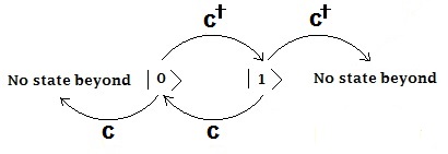
${\displaystyle {\hat {c}}^{\dagger }|0\rangle =|1\rangle }$

${\displaystyle ({\hat {c}}^{\dagger })^{2}|0\rangle ={\hat {c}}^{\dagger }|1\rangle =0}$

つまり最大占有数は1で、1個以上のフェルミ粒子は同じ状態を占有できない。

逆に${\displaystyle |1\rangle }$にくり返し消滅演算子を作用させると、${\displaystyle \{{\hat {c}},{\hat {c}}\}=2({\hat {c}})^{2}=0}$より

${\displaystyle {\hat {c}}|1\rangle =|0\rangle }$

${\displaystyle ({\hat {c}})^{2}|1\rangle ={\hat {c}}|0\rangle =0}$

つまり粒子数は0以下になれない。この${\displaystyle |0\rangle ,|1\rangle }$をフェルミ粒子におけるフォック状態と呼ぶ。

ボース粒子の場合と同様に、この場合も粒子的な解釈を行うことができる。ただし粒子の生成は1つまでしかできない。

同種粒子の不可弁別性

1つのモードでのフォック状態を合成し、2つ以上のモード（多重モード）でのフォック状態を作る。このフォック状態は、同種粒子の不可弁別性を満たすような形でなければならない。

2つのモードの場合

合成した固有状態に交換演算子${\displaystyle {\hat {P}}}$が作用すると、ボース粒子の場合は対称的、フェルミ粒子の場合は反対称的になければならない^[2]。

たとえばテンソル積表現での2粒子系においては次のようになる。

${\displaystyle {\hat {P}}\left|x_{1},x_{2}\right\rangle =\left|x_{2},x_{1}\right\rangle }$

2つの同種粒子のフォック状態${\displaystyle |1_{1},1_{2}\rangle }$について、次の不可弁別性が成り立つ。よって

• ボース粒子では${\displaystyle |1_{1},1_{2}\rangle =+|1_{2},1_{1}\rangle }$
• フェルミ粒子では${\displaystyle |1_{1},1_{2}\rangle =-|1_{2},1_{1}\rangle }$

となる^[3]:191。

証明

任意の終状態${\displaystyle |f\rangle }$、演算子${\displaystyle {\hat {\mathbb {O} }}}$とすると、 ${\displaystyle \left|\langle f|{\hat {\mathbb {O} }}|1_{1},1_{2}\rangle \right|^{2}=\left|\langle f|{\hat {\mathbb {O} }}|1_{2},1_{1}\rangle \right|^{2}}$ よって、 ${\displaystyle \langle f|{\hat {\mathbb {O} }}|1_{1},1_{2}\rangle =e^{i\delta }\langle f|{\hat {\mathbb {O} }}|1_{2},1_{1}\rangle }$ であり、 ボース粒子のときは${\displaystyle e^{i\delta }=+1}$ フェルミ粒子のときは${\displaystyle e^{i\delta }=-1}$ である。${\displaystyle \langle f|}$と${\displaystyle {\hat {\mathbb {O} }}}$は任意であるため、 ボース粒子では${\displaystyle |1_{1},1_{2}\rangle =+|1_{2},1_{1}\rangle }$ フェルミ粒子では${\displaystyle |1_{1},1_{2}\rangle =-|1_{2},1_{1}\rangle }$ となる。

ここで数演算子は、ボース粒子とフェルミ粒子を区別せずに（つまり対称性を考慮せずに）粒子を数えるだけの演算子であることに注意。 この２種類の粒子の差を見るには、生成消滅演算子が必要となる。

このように複数の同種モードがある場合、ボース粒子のフォック状態は対称性を、フェルミ粒子のフォック状態は反対称性を持たなければならない。 これらの性質を満たすため、以下で述べるように、多重モードのフォック状態をテンソル積を用いて構成する。 テンソル積は、粒子がフェルミ粒子かボース粒子かによって、基となる1粒子ヒルベルト空間の交代積または対称積でなければならない。

多重モードのボース粒子フォック状態

生成消滅演算子の導入

この新しいフォック空間表現では、同じ対称性の性質を表現しなければならない。

そのため各モード${\displaystyle i}$のボース粒子の生成消滅演算子を、以下の交換関係を満たす演算子${\displaystyle {\hat {b}}_{i}^{\dagger }}$、${\displaystyle {\hat {b}}_{i}}$として定義する^[2]。

${\displaystyle [{\hat {b}}_{i},{\hat {b}}_{j}^{\dagger }]\equiv {\hat {b}}_{i}{\hat {b}}_{j}^{\dagger }-{\hat {b}}_{j}^{\dagger }{\hat {b}}_{i}=\delta _{ij}}$

${\displaystyle [{\hat {b}}_{i}^{\dagger },{\hat {b}}_{j}^{\dagger }]=[{\hat {b}}_{i},{\hat {b}}_{j}]=0}$

ここで${\displaystyle \delta _{ij}}$はクロネッカーのデルタである。生成消滅演算子はエルミート演算子ではない^[2]。

生成消滅演算子がエルミート演算子ではない証明

フォック状態${\displaystyle |\cdots ,n_{l},\cdots \rangle }$で消滅演算子をはさむと ${\displaystyle \langle \cdots ,n_{l},\cdots |b_{l}|\cdots ,(n_{l}-1),n_{l},(n_{l}+1),\cdots \rangle ={\sqrt {n_{l}}}\langle \cdots ,n_{l},\cdots |\cdots (n_{l}-1),(n_{l}-1),(n_{l}+1),\cdots \rangle }$ 一方で生成演算子をはさむと、 ${\displaystyle =\langle \cdots ,n_{l},\cdots |b_{l}^{\dagger }|\cdots ,(n_{l}-1),n_{l},(n_{l}+1),\cdots \rangle ={\sqrt {n_{l}+1}}\langle \cdots ,n_{l}-1\cdots |\cdots ,(n_{l}-1),(n_{l}+1),(n_{l}+1),\cdots \rangle }$ よって生成(消滅)演算子のエルミート共役は、自分自身にはならない。よってエルミート演算子ではない。 生成演算子のエルミート共役は消滅演算子であり、消滅演算子のエルミート共役は生成演算子である[4]。:45

粒子数演算子

各モードの粒子数演算子を次のように定義する。

${\displaystyle {\hat {N}}_{i}\equiv {\hat {b}}_{i}^{\dagger }{\hat {b}}_{i}}$

これはエルミート演算子である。この固有値・固有ベクトルは以下を満たす。

${\displaystyle {\hat {N}}_{i}|n_{i}\rangle =n_{i}|n_{i}\rangle }$

また全数演算子を、各モード${\displaystyle i}$の数演算子の和として定義する。

${\displaystyle {\hat {n}}=\sum _{i}{\hat {n}}_{i}}$

状態のテンソル積

多重モードにおけるフォック状態${\displaystyle |n_{1},n_{2},\cdots ,n_{i},\cdots \rangle }$を、全数演算子の固有ベクトルと定義する。固有値は全てのモードの粒子数（占有数）の和である。

${\displaystyle {\hat {n}}|n_{1},n_{2},\cdots ,n_{i},\cdots \rangle =\left(\sum _{i}n_{i}\right)|n_{1},n_{2},\cdots ,n_{i},\cdots \rangle }$

多重モードフォック状態は、各モードでの${\displaystyle |n_{i}\rangle }$ の直積（テンソル積）で表される。

${\displaystyle |n_{1},n_{2},\cdots ,n_{i},\cdots \rangle \equiv |n_{1}\rangle |n_{2}\rangle \cdots |n_{i}\rangle \cdots }$

ここで各モードにおける粒子的な解釈を行うことで、多重モード全体の状態を各モードの粒子数（あるいは占有数）を用いて表すことができる。

生成消滅演算子の作用

多重モードのフォック状態におけるそれぞれの生成消滅演算子は、それ自身のモードにのみ作用する。たとえば${\displaystyle {\hat {b}}_{i}}$と${\displaystyle {\hat {b}}_{i}^{\dagger }}$は、${\displaystyle |n_{i}\rangle }$にだけ作用する^[2]。

${\displaystyle {\begin{aligned}{\hat {b}}_{i}|n_{1},n_{2},\cdots ,n_{i},\cdots \rangle &={\sqrt {n_{i}}}|n_{1},n_{2},\cdots ,n_{i}-1,\cdots \rangle \\{\hat {b}}_{i}^{\dagger }|n_{1},n_{2},\cdots ,n_{i},\cdots \rangle &={\sqrt {n_{i}+1}}|n_{1},n_{2},\cdots ,n_{i}+1,\cdots \rangle \end{aligned}}}$

つまり生成消滅演算子の多重モード状態への作用は、それら自身のモードの粒子数（あるいは占有数）を１だけ増加または減少させるだけである。異なるモードに対応する演算子はヒルベルト空間の異なる部分空間に作用する。

たとえば、

• 真空状態(どの状態にも粒子が無い状態）${\displaystyle |0_{1},0_{2},\cdots ,0_{i},\cdots \rangle }$にモード${\displaystyle i}$の生成消滅演算子が作用すると^[2]、

${\displaystyle {\begin{aligned}{\hat {b}}_{i}^{\dagger }|0_{1},0_{2},\cdots ,0_{i},\cdots \rangle &=|0_{1},0_{2},\cdots ,1_{i},\cdots \rangle \\{\hat {b}}_{l}|0_{1},0_{2},\cdots ,0_{i},\cdots \rangle &=0\end{aligned}}}$

• 生成演算子を真空状態に作用させることで、どんなフォック状態も作ることができる。

${\displaystyle |n_{1},n_{2},\cdots \rangle ={\frac {(b_{1}^{\dagger })^{n_{1}}}{\sqrt {n_{1}!}}}{\frac {(b_{2}^{\dagger })^{n_{2}}}{\sqrt {n_{2}!}}}\cdots |0_{1},0_{2},\cdots \rangle }$

数演算子の作用

i番目のモードの粒子数演算子${\displaystyle {\hat {N}}_{i}}$は、ボース粒子フォック状態に以下のように作用する^[2]。

${\displaystyle {\hat {N}}_{i}|n_{1},n_{2},\cdots ,n_{i},\cdots \rangle =n_{i}|n_{1},n_{2},\cdots ,n_{i},\cdots \rangle }$

つまりフォック状態も粒子数演算子の固有ベクトルになっている。

フォック状態は全粒子数の固有状態であるため、全粒子数の測定値の分散は${\displaystyle \operatorname {Var} ({\hat {N}})=0}$となる。すなわちフォック状態における全粒子数の測定は、常にゆらぎが無く確定値を与える。 よって、

${\displaystyle {\hat {N}}=\sum _{i}{\hat {N}}_{i}}$

数演算子と交換するハミルトニアン

各モード間の相互作用が無い系を考える。この系の全ハミルトニアン${\displaystyle {\hat {H}}}$は、各モードのハミルトニアン${\displaystyle {\hat {H}}_{i}}$の和で表される。

${\displaystyle {\hat {H}}=\sum _{i}{\hat {H}}_{i}}$

全ハミルトニアンと全数演算子は交換する。よって多重モードフォック状態は多重モードハミルトニアンの固有状態でもある（同時固有状態）。

${\displaystyle {\hat {H}}|n_{1},n_{2},\cdots ,n_{i},\cdots \rangle =\left(\sum _{i}\hbar \omega \left(n_{i}+{\frac {1}{2}}\right)\right)|n_{1},n_{2},\cdots ,n_{i},\cdots \rangle }$

各モードで考えると、モード${\displaystyle i}$のハミルトニアン${\displaystyle {\hat {H}}_{i}}$の固有状態は、粒子数演算子${\displaystyle {\hat {N}}_{i}}$の固有状態にもなっている（厳密にはさらに位相因子を選択しなければならない）。

ここで粒子的な解釈を行うことで、${\displaystyle {\hat {N}}_{i}}$の固有状態に対応する固有値${\displaystyle n_{i}}$は、モード${\displaystyle i}$のハミルトニアン${\displaystyle {\hat {H}}_{i}}$の${\displaystyle n}$番目の固有状態${\displaystyle |\psi _{n}\rangle }$における粒子数を与える。

フォック空間

フォック状態はエルミート演算子である粒子数演算子の固有ベクトルであるため、正規直交基底をなす。 このフォック状態（とそれらの線形結合）から成る空間をフォック空間という。 フォック空間での基底であるフォック状態は、「占有数基底」とも呼ばれる。 フォック空間は、それぞれの粒子数におけるテンソル積ヒルベルト空間の直和となる。

フォック空間のベクトルの中で、粒子数が異なる状態の重ね合わせであるもの（たとえばコヒーレント状態など）は、数演算子の固有状態ではないためフォック状態ではない。よってフォック空間の全てのベクトルが「フォック状態」と呼ばれる訳ではない。

粒子数 (N)	ボース粒子フォック空間の基底[5]:11
0	${\displaystyle |0,0,0,\cdots \rangle }$
1	${\displaystyle |1,0,0,\cdots \rangle }$, ${\displaystyle |0,1,0,\cdots \rangle }$,${\displaystyle |0,0,1,\cdots \rangle }$,...
2	${\displaystyle |2,0,0,\cdots \rangle }$, ${\displaystyle |1,1,0,\cdots \rangle }$,${\displaystyle |0,2,0,\cdots \rangle }$,...
...	...

ボース粒子フォック状態の対称性

ボース粒子フォック状態が粒子の交換によって対称性を示すことを確認する。

ここで２つの状態間の粒子の交換は、ある状態でのある粒子を消滅させ、別の状態での粒子を生成させることで行われる。 フォック状態${\displaystyle |\cdots ,n_{m},\cdots ,n_{l},\cdots \rangle }$ から出発して状態${\displaystyle l}$から状態${\displaystyle m}$への粒子をシフトさせたい場合は、交換関係より${\displaystyle {\hat {b}}_{m}^{\dagger }{\hat {b}}_{l}={\hat {b}}_{l}{\hat {b}}_{m}^{\dagger }}$であるため、

${\displaystyle {\begin{aligned}{\hat {b}}_{m}^{\dagger }{\hat {b}}_{l}|\cdots ,n_{m},\cdots ,n_{l},\cdots \rangle &={\hat {b}}_{l}{\hat {b}}_{m}^{\dagger }|\cdots ,n_{m},\cdots ,n_{l},\cdots \rangle \\&={\sqrt {n_{m}+1}}{\sqrt {n_{l}}}|\cdots ,n_{m}+1,\cdots ,n_{l}-1,\cdots \rangle \end{aligned}}}$

よってボース粒子フォック状態は粒子の交換において対称的である。

多重モードのフェルミ粒子フォック状態

フェルミ粒子の生成消滅演算子

フェルミ粒子の反対称性を保持するために、フェルミ粒子の生成消滅演算子を導入する。 フェルミ粒子フォック状態 ${\displaystyle |n_{1},n_{2},\cdots ,n_{l},\cdots \rangle }$に生成演算子を次のように作用させる。

${\displaystyle {\hat {c}}_{l}^{\dagger }|n_{1},n_{2},\cdots ,n_{l},\cdots \rangle ={\sqrt {n_{l}+1}}|n_{1},n_{2},\cdots ,n_{l}+1,\cdots \rangle }$ ^[2]

消滅演算子は次のように作用する。

${\displaystyle {\hat {c}}_{l}|n_{1},n_{2},\cdots ,n_{l},\cdots \rangle ={\sqrt {n_{l}}}|n_{1},n_{2},\cdots ,n_{l}-1,\cdots \rangle }$ ^[2]

これら２つの演算子の作用は反対称的に行われる（後述）。

演算子の反交換関係

フェルミ粒子系における生成消滅演算子の反交換関係は、

${\displaystyle \{{\hat {c}}_{i},{\hat {c}}_{j}^{\dagger }\}\equiv {\hat {c}}_{i}{\hat {c}}_{j}^{\dagger }+{\hat {c}}_{j}^{\dagger }{\hat {c}}_{i}=\delta _{ij}}$

${\displaystyle \{{\hat {c}}_{i}^{\dagger },{\hat {c}}_{j}^{\dagger }\}=\{{\hat {c}}_{i},{\hat {c}}_{j}\}=0}$ ^[2]

ここで${\displaystyle {\{\ ,\ \}}}$ は反交換子、${\displaystyle \delta _{ij}}$はクロネッカーのデルタである。これらの反交換関係は、フェルミ粒子フォック状態の反対称性を表すために用いられる。

数演算子の作用

フェルミ粒子の数演算子は次のように与えられる。

${\displaystyle {\hat {N}}_{l}={\hat {c}}_{l}^{\dagger }{\hat {c}}_{l}}$

これがフェルミ粒子フォック状態に作用すると、

${\displaystyle {\hat {N}}_{l}|n_{1},n_{2},\cdots ,n_{l},\cdots \rangle =n_{l}|n_{1},n_{2},\cdots ,n_{l},\cdots \rangle }$ ^[2]

最大占有数

生成消滅演算子や数演算子の作用はボース粒子の場合と同じであるように見えるが、フェルミ粒子フォック状態の最大占有数から違いが生じる。 上述の２つのフェルミ粒子の例を拡張し、 次のように置換演算子のある特定の和を固有ケットのテンソル積に適用することで、 フェルミ粒子フォック状態${\displaystyle |n_{1},n_{2},\cdots ,n_{l},\cdots \rangle }$が得られることをまず確かめておかなければならない。

${\displaystyle |n_{1},n_{2},\cdots ,n_{l},\cdots \rangle =S_{-}|i_{1},i_{2},\cdots ,i_{l},\cdots \rangle ={\frac {1}{\sqrt {N!}}}{\begin{vmatrix}|i_{1}\rangle _{1}&\cdots &|i_{1}\rangle _{N}\\\vdots &\ddots &\vdots \\|i_{N}\rangle _{1}&\cdots &|i_{N}\rangle _{N}\end{vmatrix}}}$ ^[6]:16

この行列式はスレーター行列式と呼ばれる^[要出典]。 もし1粒子状態でも同じものがあればスレーター行列式の2つの行は同じであり、行列式は0になる。 これは2つの同種フェルミ粒子が同じ状態を占めないことをあらわしている。 よっていかなる単一状態の占有数も0または1のどちらかである。 フェルミ粒子フォック状態に関連する固有値${\displaystyle {\hat {N}}_{l}}$は0または1である。

フェルミ粒子フォック空間の基底

粒子数 (N)	フェルミ粒子フォック空間の基底[5]:11
0	${\displaystyle |0,0,0,\cdots \rangle }$
1	${\displaystyle |1,0,0\cdots \rangle }$, ${\displaystyle |0,1,0,\cdots \rangle }$, ${\displaystyle |0,0,1,\cdots \rangle }$,...
2	${\displaystyle |1,1,0,\cdots \rangle }$, ${\displaystyle |0,1,1,\cdots \rangle }$, ${\displaystyle |0,1,0,1,\cdots \rangle }$,${\displaystyle |1,0,1,0,\cdots \rangle }$,...
...	...

具体的なフォック状態への作用

${\displaystyle |n_{1},n_{2},\cdots ,n_{\beta },n_{\alpha },\cdots \rangle }$で表される多重モードフェルミ粒子フォック状態では、

${\displaystyle {\hat {c}}_{\alpha }|n_{1},n_{2},\cdots ,n_{\beta },n_{\alpha },\cdots \rangle =(-1)^{\sum _{\beta <\alpha }n_{\beta }}|n_{1},n_{2},\cdots ,n_{\beta },1-n_{\alpha },\cdots \rangle }$

ここで${\displaystyle (-1)^{\sum _{\beta <\alpha }n_{\beta }}}$は、ヨルダン-ウィグナーストリングと呼ばれ、含まれる1粒子状態の順序に依存し、全ての前に来る状態のフェルミ粒子占有数を足し合わせる。^[4]:88

フェルミ粒子フォック状態の反対称性

交換演算子のもとでのフェルミ粒子状態の反対称性は、反交換関係によるものである。 ここでは2つの状態間の粒子の交換は、ある状態のある粒子を消滅させ、別の粒子を生成させることで行われる。 フォック状態${\displaystyle |n_{1},n_{2},\cdots ,n_{m}\cdots ,n_{l},\cdots \rangle }$から出発して状態${\displaystyle l}$から状態 ${\displaystyle m}$へ粒子をシフトさせたい場合、反交換関係より${\displaystyle {\hat {c}}_{m}^{\dagger }{\hat {c}}_{l}=-{\hat {c}}_{l}{\hat {c}}_{m}^{\dagger }}$であるため、

${\displaystyle {\hat {c}}_{m}^{\dagger }{\hat {c}}_{l}|n_{1},n_{2},\cdots ,n_{m},\cdots ,n_{l},\cdots \rangle ={\sqrt {n_{m}+1}}{\sqrt {n_{l}}}|n_{1},n_{2},\cdots ,n_{m}+1,\cdots ,n_{l}-1,\cdots \rangle }$

しかし、

${\displaystyle {\begin{aligned}{\hat {c}}_{l}{\hat {c}}_{m}^{\dagger }|n_{1},n_{2},\cdots ,n_{m},\cdots ,n_{l},\cdots \rangle &=-{\hat {c}}_{m}^{\dagger }{\hat {c}}_{l}|n_{1},n_{2},\cdots ,n_{m},\cdots ,n_{l},\cdots \rangle \\&=-{\sqrt {n_{m}+1}}{\sqrt {n_{l}}}|n_{1},n_{2},\cdots ,n_{m}+1,\cdots ,n_{l}-1,\cdots \rangle \end{aligned}}}$

よってフェルミ粒子フォック状態は、粒子の交換において反対称性である。

フォック状態は一般的にエネルギー固有状態では無い

第二量子化理論では、ハミルトニアン密度関数は次のように与えられる。

${\displaystyle {\mathfrak {H}}={\frac {1}{2m}}\nabla _{i}\psi ^{*}(x)\nabla _{i}\psi (x)}$ ^[3]:189

全ハミルトニアンは、次のように与えられる。

${\displaystyle {\mathcal {H}}=\int d^{3}x\,{\mathfrak {H}}=\int d^{3}x\psi ^{*}(x)\left(-{\tfrac {\nabla ^{2}}{2m}}\right)\psi (x)\quad (\therefore {\mathfrak {H}}=-{\tfrac {\nabla ^{2}}{2m}})}$

自由粒子のシュレーディンガー方程式^[3]:189 は、

${\displaystyle {\mathfrak {H}}\psi _{n}^{(+)}(x)=-{\tfrac {\nabla ^{2}}{2m}}\psi _{n}^{(+)}(x)=E_{n}^{0}\psi _{n}^{(+)}(x)}$

この解は直交性を満たす。

${\displaystyle \int d^{3}x\,\psi _{n}^{(+)^{*}}(x)\psi _{n'}^{(+)}(x)=\delta _{nn'}}$

また消滅演算子を${\displaystyle {\hat {a}}_{n}}$として、次の関係がある。

${\displaystyle \psi (x)=\sum _{n}{\hat {a}}_{n}\psi _{n}^{(+)}(x)}$

よって、

${\displaystyle \therefore {\mathcal {H}}=\sum _{n,n'}\int d^{3}x\,{\hat {a}}_{n'}^{\dagger }\psi _{n'}^{(+)^{*}}(x){\mathfrak {H}}{\hat {a}}_{n}\psi _{n}^{(+)}(x)}$

相互作用しない粒子においてのみ、${\displaystyle {\mathfrak {H}}}$と${\displaystyle {\hat {a}}_{n}}$が交換する。しかし一般の場合にはこれらは交換しない。 相互作用しない粒子では、

${\displaystyle {\mathcal {H}}=\sum _{n,n'}\int d^{3}x\,{\hat {a}}_{n'}^{\dagger }\psi _{n'}^{(+)^{*}}(x)E_{n}^{0}\psi _{n}^{(+)}(x){\hat {a}}_{n}=\sum _{n,n'}E_{n}^{0}{\hat {a}}_{n'}^{\dagger }{\hat {a}}_{n}\delta _{nn'}=\sum _{n}E_{n}^{0}{\hat {a}}_{n}^{\dagger }{\hat {a}}_{n}=\sum _{n}E_{n}^{0}{\hat {N}}}$

これらが交換しない場合、ハミルトニアンは上述の表現を持たない。 よって一般的にフォック状態は系のエネルギー固有状態ではない。

真空ゆらぎ

真空状態${\displaystyle |0\rangle }$は最低エネルギーの状態で、${\displaystyle {\hat {a}}}$と${\displaystyle {\hat {a}}^{\dagger }}$の期待値はこの状態では0になる。

${\displaystyle {\hat {a}}|0\rangle =\langle 0|{\hat {a}}^{\dagger }=0}$

電磁場とベクトルポテンシャルは同じ一般形のモード展開を持つ。

${\displaystyle F({\boldsymbol {r}},t)=\varepsilon ae^{i{\boldsymbol {\psi }}\cdot {\boldsymbol {r}}-\omega t}+hc}$

これらの場の演算子の期待値が真空状態では0になることを見るのは簡単である。

${\displaystyle \langle 0|F|0\rangle =0}$

しかし、これらの場の演算子の二乗の期待値は0ではないことを示すことができる。 このように0アンサンブル平均についての場におけるゆらぎが存在する。 これらの真空ゆらぎは、量子光学におけるラムシフトなど多くの興味深い現象の原因となる。

単一フォトン状態の源

単一フォトンは、シングルエミッター(原子、窒素-空孔中心^[7]、 量子ドット^[8])を用いてごく普通に生成される。 しかしこれらの源はいつも効率的であるとは限らず(要求に応じた単一フォトンを実際に得る確率は低い)、しばしば複雑で、実験環境からは適さない。 非決定的ふるまいを犠牲にして、これらの問題を克服する別の源が一般的に用いられる。 歓迎された単一フォトン源は確率的２フォトン源で、そこからペアが分かれ、1フォトンの検出は残りのフォトンの存在を歓迎する。 これらの源はたとえば周期的に分極したニオブ酸リチウム(自発的パラメトリック下方変換)やシリコン(自発的四波混合)など、通常いくつかの材料の非線形光学作用に依存している。

非古典的ふるまい

フォック状態のスダルシャン・グラウバーのP表現（英語版）は、これらの状態が純粋に量子力学的な状態であり、古典的対応物は存在しないことを示している。 この表現におけるこれらの状態の${\displaystyle \varphi (\alpha )}$^[要説明]はディラックのデルタ関数の${\displaystyle 2n}$次導関数であり、よって古典的な確率分布ではない。

脚注

関連項目

• コヒーレント状態
• ハイゼンベルク極限
• 非古典光

外部リンク

• Vladan Vuletic of MIT has used an ensemble of atoms to produce a Fock state (a.k.a. single photon) source (PDF)
• Produce and measure a single photon state (Fock state) with an interactive experiment QuantumLab